
Hide
Using the vlookup function (exact)
You can download here the worksheet from this video to practice it by yourself!
Vlookup Tutorial For Beginners
The video above shows how to use Excel's vlookup to fill in data for you:You will enter the student's score, and the spreadsheet will automatically fill in the corresponding letter grade for this score (for Example 70 will give the letter "C" letter), and the corresponding verbal description (in our example: "Below average").
How will vlookup know how to do it? Well, it will take the score you enter, and will look it up the table's first column, and retrieve the value that is written next to it.
In our first example, it will look for the value 70 in the table, and will retrieve the letter C which is in the 2nd column in the table.
You can download the spreadsheet used in this video by clicking the "Try it yourself" button above.
Building the function step by step:
1. Type the following code: =vlookup(2. Type the address of the cell containing the value to look for in the table.
3. Type the range of the table to look inside, (or better: Name the table before starting with the function, and type now its name). Remember: don’t include the table’s heading row.
4. Type the column number from which you want to retrieve the result.
5. Type the word FALSE which means: “Please find me exactly the value of the cell mentioned in step 2. (Don’t round it down to the closest match)”.
6. Close the bracket and hit the [Enter] key.
Note: The function will always look for the value mentioned on step 2 only on the first column (the utmost left column) of the table.
Vlookup Examples:
Let’s assume you are using the following Excel worksheet.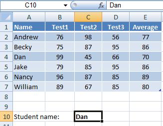
(If you wish, you can download this worksheet here.)
=vlookup(C10,A2:E7,2,FALSE)
In words: Look for the value of cell C10 inside table located at A2:E7, and retrieve me the value on the 2’nd column. Please find me exactly what’s in cell C10.
The value of the above formula will be: 99 (on Dan’s row, the second column).
The value of the above formula will be: 99 (on Dan’s row, the second column).
Copying and replicating the function
If you plan on copying the vlookup function (either by “copy” and “paste” or by dragging it with the fill handle), make sure to set the table’s address with absolute reference (e.g. $A$2:$E$7). But it would be easier instead to simply name the table, as in the following example.You can name the range A2:E7 by selecting it, and typing the name in the name box. (The name box is located on the top-left corner of the screen).
Let’s assume you named it studentsTable (spaces are not allowed, but you may use underscores).
=vlookup(c10,studentsTable,3,false)
In words: Look for the value in cell C10 inside studentsTable, and retrieve the value from the table’s 3’rd column. Please find me exactly what’s in cell C10.
The value of the above function will be: 45 (on Dan’s row, the value in the third column of the table).
The value of the above function will be: 45 (on Dan’s row, the value in the third column of the table).
Troubleshoot (advanced usage with more functions)
(You should be familiar with the IF function to understand this section)If the vlookup doesn’t find a match, it will write the following code: #N/A. That's quite annoying.
You can overcome this code, and choose what do display in this case, by using the IF function with the ISNA() function.
The isna() function gives "true" if the vlookup inside it does'nt find any match. So we'll use it as the condition part of an IF function.
Look at the following example:
=if(isna(vlookup(c10,studentsTable,3,false)),”didn’t find any match”, vlookup(c10,studentsTable,3,false))
In words: if the vlookup function gives us the #N/A code, then write “didn’t find any match”, else compute the vlookup function.
Explanation:
The 3 parts of the above IF function are:
1. isna(vlookup(c10,studentsTable,3,false))
2. “didn’t find any match”
3. vlookup(c10,studentsTable,3,false)
The first part is a condition, which says: Does the vlookup function gives us the #N/A code?
If it does, write “didn’t find any match”, otherwise compute the vlookup function.
Tip:
Instead of the part “did'nt find any match”, you can put only double quotation marks “” which will leave the cell empty in case no match is found:
=if(isna(vlookup(c10,studentsTable,3,false)),””, vlookup(c10, studentsTable,3,false))
or let it show the value 0 in case of no match:
=if(isna(vlookup(c10,studentsTable,3,false)),0, vlookup(c10, studentsTable,3,false))
You can see a demonstration of using the IF with ISNA() function and read more about it over here.