Learn how to create a drop down list inside an Excel cell
A drop down list enables you to choose a value from a list, instead of typing it.
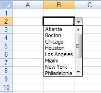
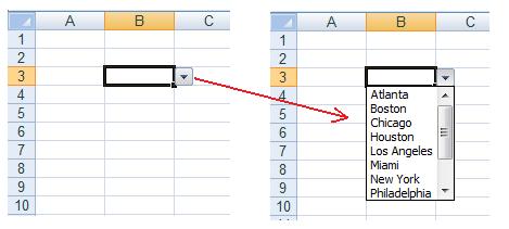
Here is an example of a drop down list that was created in cell B3. Clicking the small arrow next to the cell, will open the list:
Creating a drop down list in Excel: Step by Step
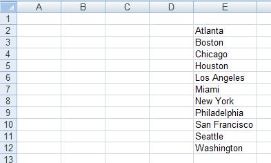
1. Write the list somewhere inside the worksheet. It is recommended to have it sorted alphabetically in ascending order, because this is the order in which they will appear in the drop down list.
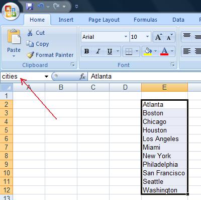
2. Name the list, by selecting its range and writing its name in the name box. In this example we named it "cities":
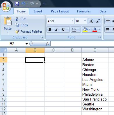
3. Select the cell in which you want the drop down list to appear. In this example we selected cell B2:
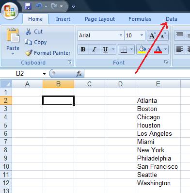
4. Choose the "Data" tab from the ribbon.
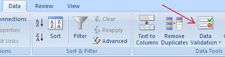
5. Click the "Data Validation" button.
It will look like one of the two following examples, depending on your screen resolution:
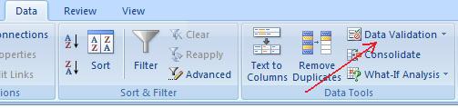
OR:
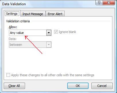
6. A dialog box will appear. Click the words "Any value" and choose "List".
7. Click inside the "Source" text field, and write =the name you gave to the list (in our example: =cities).
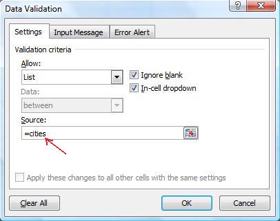
8. Click the OK button.
Done! Now you have a drop down list inside your selected cell.